vector arithmetic
//+ addition ;
v1 = {a,2,c}+{1,b,3};
show v1;
save as addition;
//- addition ;
v1 = {a,b,c} - {0, 0, 0};
show v1;
save as subtraction;
// v - v = 0 ;
v1 = {a,b,c} ; v2 = v1 - v1;
show v1 also v2;
save as subtraction;
// v1 + v2 = v2 + v1 ;
v1 = {a,b,c} ; v2 = {1,2,3};
v3 = v1+v2; v4 = v2+v1;
v5 = v3 == v4;
show v1 also v2 also v3 also v4 also v5;
save as subtraction;
// (v1 + v2) + v3 = v1 + (v2 + v3);
v1 = {a,b,c} ; v2 = {1,2,3}; v3 = {p,q,r};
//fist add v1 and v2 then v3; tmp1 = v1+v2;
v5 = tmp1 +v3;
//first add v2 and v3 then v1; tmp2 = v2 +v3;
v4 = v1 + tmp2;
v6 = v4 == v5;
show v1 also v2 also v3 also v4 also v5 also v6;
save as addition;
SCALE
v = u * {a, b, c, d, e, f};
show v;
save as scale;
v = u * {a, b, c, d, e, f};
show v;
save as scale;
v1 = {x, y}; v2 = v1 + v1; v3 = 2 * v1;
show v2 also v3;
save as scale;
v1 = {x, y}; v2 = v1 + v1 + v1; v3 = 3 * v1;
show v2 also v3;
save as scale;
v = t *{a, b, c, d, e, f} * s;
show v;
save as scale;
v = (s+t) * {a, b, c, d, e, f};
show v;
show expand[v];
show simplify[v];
save as scale;
v = 0 * {a, b, c, d, e, f};
show v;
save as scale;
v = 1 * {a, b, c, d, e, f};
show v;
save as scale;
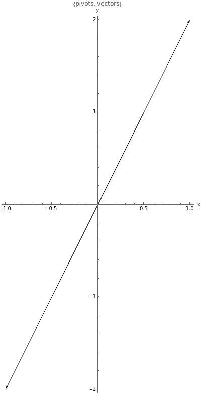
NEGAGIVE
v1 = {1,2}; v2 = -1*v1; //v2 = -v1;
//list of pivots; pivots = {{0,0}, {0,0}}; //list of vectors; vectors = {v1,v2};
vectorplot pivots vectors;
save as scale;
In modern geometry all geometrical forms are defined by algebraic means and methods. For example a circle is defined by the algebraic tokens (symbols) x and y and = equality operator and r the token for radius in this equation:
x2 + y2 = r2
The Left Hand Side measures the distance between the point (x, y) and the origin of the circle namely (0,0) and the Right Hand Side r is the radius.
If you like to move your circle to another point (a,b) then the new Equational Form of the circle is:
(x - a)2 + (y - b)2 = r2
Now imagine you had never seen such algebraic use and no idea what any of that Equational Form supposed to mean and yet you are compelled to visualize and study the said circle. What would you do?
Instance [ ]
Use the Free Form function Instance [ ] as follows:
- Pass the Equational Form as an argument to Instance [ ] to compute a sample (x, y) values that satisfy the Equational Form
- Pass the number of such instances
Example
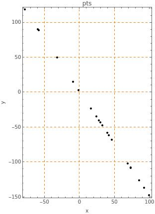
linear = 3*x+2*y;
pts = instance [ linear == 3 ,20];
show pts;
pointplot pts;
save as line;
'==': Boolean Equality operator or ==
As you can see the coordinates x and y have a range of ±100 which is too wide to study and you like to study the geometry of this line around the origin at (0,0).
All you need to do is to limit the range of x and y say around ±5
linear = 3*x+2*y;
pts = instance [ linear == 3 and -5<x<5 and -5<y<5 ,20];
show pts;
pointplot pts;
save as line_enclosed;
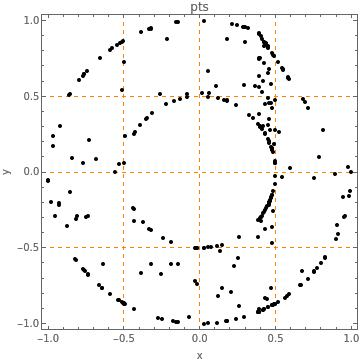
Enclose a region between our line above and an annulus which is nothing more than a Disk cutout of a larger Disk or
r12 ≦ x2 + y2 ≦ r22
radius=norm[{x,y}];
linear = 3*x+2*y;
pts = instance [linear <= 3 and 0.5<=radius <=1 ,300];
//show pts;
pointplot pts;
save as cropped_anulus;