vector arithmetic

//+ addition ;

v1 = {a,2,c}+{1,b,3};

show v1;

save as addition;

//- addition ;

v1 = {a,b,c} - {0, 0, 0};

show v1;

save as subtraction;

// v - v = 0 ;

v1 = {a,b,c} ; v2 = v1 - v1;

show v1 also v2;

save as subtraction;

// v1 + v2 = v2 + v1 ;

v1 = {a,b,c} ; v2 = {1,2,3};

v3 = v1+v2; v4 = v2+v1;

v5 = v3 == v4;

show v1 also v2 also v3 also v4 also v5;

save as subtraction;

// (v1 + v2) + v3 = v1 + (v2 + v3);

v1 = {a,b,c} ; v2 = {1,2,3}; v3 = {p,q,r};

//fist add v1 and v2 then v3; tmp1 = v1+v2;

v5 = tmp1 +v3;

//first add v2 and v3 then v1; tmp2 = v2 +v3;

v4 = v1 + tmp2;

v6 = v4 == v5;

show v1 also v2 also v3 also v4 also v5 also v6;

save as addition;

SCALE

v = u * {a, b, c, d, e, f};

show v;

save as scale;

v = u * {a, b, c, d, e, f};

show v;

save as scale;

v1 = {x, y}; v2 = v1 + v1; v3 = 2 * v1;

show v2 also v3;

save as scale;

v1 = {x, y}; v2 = v1 + v1 + v1; v3 = 3 * v1;

show v2 also v3;

save as scale;

v = t *{a, b, c, d, e, f} * s;

show v;

save as scale;

v = (s+t) * {a, b, c, d, e, f};

show v;

show expand[v];

show simplify[v];

save as scale;

v = 0 * {a, b, c, d, e, f};

show v;

save as scale;

v = 1 * {a, b, c, d, e, f};

show v;

save as scale;

NEGAGIVE

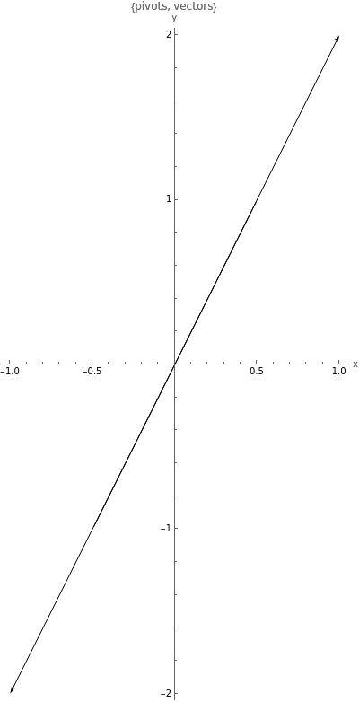
v1 = {1,2}; v2 = -1*v1; //v2 = -v1;

//list of pivots; pivots = {{0,0}, {0,0}}; //list of vectors; vectors = {v1,v2};

vectorplot pivots vectors;

save as scale;

In modern geometry all geometrical forms are defined by algebraic means and methods. For example a circle is defined by the algebraic tokens (symbols) x and y and = equality operator and r the token for radius in this equation:

x² + y² = r²

The Left Hand Side measures the distance between the point (x, y) and the origin of the circle namely (0,0) and the Right Hand Side r is the radius.

If you like to move your circle to another point (a,b) then the new Equational Form of the circle is:

(x - a)² + (y - b)² = r²

Now imagine you had never seen such algebraic use and no idea what any of that Equational Form supposed to mean and yet you are compelled to visualize and study the said circle. What would you do?

Instance [ ]

Use the Free Form function Instance [ ] as follows:

1. Pass the Equational Form as an argument to Instance [ ] to compute a sample (x, y) values that satisfy the Equational Form
2. Pass the number of such instances

Example

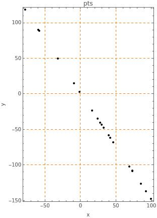
linear = 3*x+2*y;

pts = instance [ linear == 3 ,20];

show pts;

pointplot pts;

save as line;

'==': Boolean Equality operator or ==

As you can see the coordinates x and y have a range of ±100 which is too wide to study and you like to study the geometry of this line around the origin at (0,0).

All you need to do is to limit the range of x and y say around ±5

linear = 3*x+2*y;

pts = instance [ linear == 3 and -5<x<5 and -5<y<5 ,20];

show pts;

pointplot pts;

save as line_enclosed;

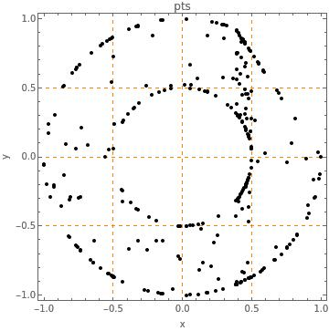
Enclose a region between our line above and an annulus which is nothing more than a Disk cutout of a larger Disk or

r₁² ≦ x² + y² ≦ r₂²

radius=norm[{x,y}];

linear = 3*x+2*y;

pts = instance [linear <= 3 and 0.5<=radius <=1 ,300];

//show pts;

pointplot pts;

save as cropped_anulus;

v1 = {x, y, z};

length1 = ||v1||;

length2 = norm[v1];

show length1 also length2;

save as length;

v1 = {a, b, c, d ,e};

length = norm[v1];

show length;

save as length;

num = sqrt[r1];

r2 = num^2;

r3 = num*num;

show r2 also r3;

save as root;

v = {x,y};

show normalize[v];

save as vectors;

v={x,y,z};

res = simplify[norm[normalize[v]]];

show res;

v1 = {x, y};

v2 = s * v1;

c1 = ||v2||/||v1||;

c2 = simplify[c1];

show v2 also c1 also c2;

save as norm_vs_scale;

v2 = s * v1: Scale the vector v1 by scale factor s.
c1 = ||v2|| / ||v1|| : Compute the ratio of norm or length of the scaled vector v2 divided by the norm or length of the original vector v1.

As the computations show, the said ratio ||v2||/||v1|| is the original s the scale factor!

In another way, ||v2|| = s * ||v1|| .

What & How & Why is Pi???

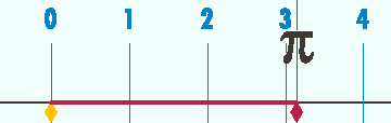
Pi (π) (/paɪ/) is a mathematical constant that is the ratio of a circle's circumference to its diameter. This produces a number, and that number is always the same. However, the number is rather strange.

The diameter is the largest chord which can be fitted inside a circle. It passes through the center of the circle.

The distance around a circle is known as the circumference.

Even though the diameter and circumference are different for different circles, the number pi remains constant: its value never changes. This is because the relationship between the circumference and diameter is always the same!!!

v = 12.36*{cos[2*pi*t], sin[2*pi*t]};

radius = simplify[ norm[v] ];

points = do[v, 40];

v2 = difference[points];

l = apply[norm, v2];

circumference = total[l];

mypi = circumference/(2*radius);

show mypi;

pointplot points;

save as pi;

v = 12.36 {cos[2 pi t], sin[2 pi t] } : parametric equation parametric_curves for the vector that spans the circle's circumference.

radius = simplify[ norm[v] ] : compute the norm of v which is the length of vector v for any value of the variable t or shown as v[t] and due to the very definition of the circle is a constant number in our case was set to 12.36.

points = do[v, 40] : repetitively do compute 40+1 points around the circle by dividing the interval [0, 1] into 40 equal partitions.

v2 = difference[points] : assume each point is represented by a vector with pivot at origin {0, 0} endpoint at {x, y, z} as was computed by the do [ ]; start with the 2nd point/vector and subtract it from the previous point/vector namely the 1st, then move to the 3rd point/vector subtract from the 2nd point/vector until you are out of point/vectors. See the output’s arrowplot, each little vector is one of the subtractions above.

See how difference works by experimenting with the very short Free Form script below:

v = {a1, a2, a3, a4};

diff = difference[v];

show diff;

save as difference;